


Contrasting Shifts in Vegetation "Greenness"
This study delves into the interannual variability (IAV) of vegetation greenness and carbon sequestration, vital for assessing ecosystem stability and climate responses. Analyzing various satellite data and models, it reveals conflicting trends in IAV, particularly in tropical regions. Uncertainty persists due to differing methodologies among remote sensing products, challenging climate change impact assessments.
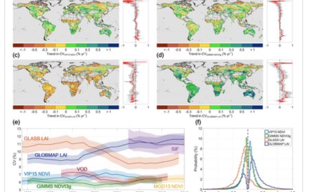
Vegetation greenness changes year to year in response to climate variability and reflects the stability of ecosystems. How the interannual variability (IAV) of vegetation greenness has changed in the past decades, however, remained uncertain with recent studies reporting conflicting IAV trends using different satellite remote sensing products. Here, we investigated the greenness IAV trends of global vegetation using multiple mainstream satellite remote sensing products. We found that the changes in greenness IAV are conflicting on half of the global vegetated surface, while the differences in background climate, greening trends and nitrogen deposition rates account for either positive or negative trends in greenness IAV on the remaining half of the vegetated surface.
Abstract
Changes in the interannual variability (IAV) of vegetation greenness and carbon sequestration are key indicators of the stability and climate sensitivities of terrestrial ecosystems. Recent studies have examined the changes in the vegetation IAV using atmospheric CO2 observations and dynamic global vegetation models (DGVMs), however, reported different and even contradictory IAV trends. Here, we investigate the changes in the IAV of vegetation greenness, quantified as coefficient of variability (CV), over the past few decades based on multiple satellite remote sensing products and DGVMs. Our results suggested that, on half of the global vegetated surface (mostly in the tropics), the CV trends detected by different satellite remote sensing products are conflicting. We found that 22.20% and 28.20% of the global vegetated surface (mostly in the non-tropical land surface) show significant positive and negative CV trends (p ≤ 0.1), respectively. Regions with higher air temperature and greater aridity tend to have increasing CV trends, whereas greater vegetation greening trend and higher nitrogen deposition lead to smaller CV trends. DGVMs generally cannot capture the CV trends obtained from satellite remote sensing products, while the inconsistency among satellite remote sensing products is likely caused by their process algorithms rather than the sensors utilized. Our study closely examines the changes in the IAV of global vegetation greenness, and highlights substantial uncertainty when using satellite remote sensing to study the response of terrestrial ecosystems to climate change.
Key Points
-
On half of the global vegetated surface, the changes in the vegetation greenness interannual variability (IAV) are conflicting
-
22.20% and 28.20% of the global vegetated surface show significant positive and negative trends of vegetation greenness IAV, respectively
-
Warmer and drier places lead to greater greenness IAV whereas greater greening trend and higher nitrogen deposition make IAV smaller
Plain Language Summary
Vegetation greenness changes year to year in response to climate variability and reflects the stability of ecosystems. How the interannual variability (IAV) of vegetation greenness has changed in the past decades, however, remained uncertain with recent studies reporting conflicting IAV trends using different satellite remote sensing products. Here, we investigated the greenness IAV trends of global vegetation using multiple mainstream satellite remote sensing products. We found that the changes in greenness IAV are conflicting on half of the global vegetated surface, while the differences in background climate, greening trends and nitrogen deposition rates account for either positive or negative trends in greenness IAV on the remaining half of the vegetated surface.
1 Introduction
Changes in the interannual variability (IAV) of vegetation greenness indicate the stability of terrestrial ecosystems (Berdugo et al., 2022; De Keersmaecker et al., 2014; Huang & Xia, 2019) and is critical for tracking the progression of vegetation-climate feedback under climate change (Alkama & Cescatti, 2016; Zeng et al., 2017). When climate variability remains unchanged, a larger IAV suggests that the vegetation is more sensitive to climate change, while a smaller IAV suggests that vegetation is less sensitive. Several recent studies have examined the IAV changes of carbon sequestration using atmospheric observations and dynamic global vegetation models (DGVMs) (Fernández-Martínez et al., 2023; Luo & Keenan, 2022) and reported an increase in the IAV from the 1950–1980s, however, they disagreed on the direction of the IAV trends from the 1980s onwards. Additionally, the conflicting evidence on the changes in climate sensitivities of vegetation greenness in recent decades (Zeng, Hu, et al., 2022; Zhang et al., 2022; Zhang et al., 2023) adds further debates to the unresolved understanding of the changes in the IAV of vegetation over the past 40 years.
Multiple factors in the global change can be linked to the changes in the IAV of vegetation activities. The greening of the earth indicates that terrestrial ecosystems hold more green leaves for carbon fluxes, which is more likely to demonstrate larger IAV in greenness and carbon fluxes. If the climate sensitivity of individual leaves remains unchanged, then climate variation would lead to a larger variation in greenness, simply because there are more leaves that can respond to climate variation. Therefore, the reasons for the greening, for example, CO2 fertilization effect and nitrogen deposition (N deposition) (Piao et al., 2015; Zhu et al., 2016) are potential factors for the changes in IAV. Aridity is another potential factor, as the droughts have been reported to either induce the changes in the trend of vegetation greenness (and therefore, a change in the IAV assuming a constant trend) (Berdugo et al., 2022), or directly enhance the variability of carbon cycle by increasing tropical extreme droughts (Luo & Keenan, 2022). Land cover and land use changes (e.g., expansion of croplands), temperature or CO2 induced the changes of respirations (Forkel et al., 2016; Piao et al., 2018), have been linked to the increase in seasonal amplitude of atmospheric CO2 (i.e., an indicator of intra-annual variability of the carbon cycle) (Gray et al., 2014), and may thus further imply the changes in the IAV of vegetation activities.
Although the changes in the vegetation IAV have been investigated and examined using atmospheric CO2 and DGVMs (Fernández-Martínez et al., 2023; Luo & Keenan, 2022), they have rarely been investigated using satellite-based observations. Two previous studies examined the changes in the temporal variability of vegetation greenness using a single satellite remote sensing product but reported different IAV trends (Chen, Chen, et al., 2019; Luo & Keenan, 2022). In this study, we used an ensemble of multiple satellite remote sensing products, covering different types of vegetation indicators, to investigate the changes in the IAV (i.e., CV; coefficient of variability) of global vegetation activities over the past 40 years. We primarily focus on the IAV of vegetation greenness including leaf area index (LAI) and normalized difference vegetation index (NDVI), but also examine other indicators, such as, solar-induced fluorescence (SIF) and vegetation optical depth (VOD). The use of CV aims to standardize the indicators, removing the differences in magnitude to ensure comparability among the results from different indicators. Beyond conducting a data intercomparison, we further collected LAI estimates from 12 DGVMs for a model-observation comparison, explored the potential factors driving the CV trends and quantified their respective contributions to the CV trends. Our study aims to improve our understanding of the IAV changes of the global vegetation greenness and identify the potential factors driving the changes in the IAV.
2 Materials and Methods
2.1 Satellite Remote Sensing Data
We used six long-term and three short-term satellite remote sensing datasets in this study, covering four types of vegetation indicators - NDVI, LAI, SIF and VOD (Table 1). These remote sensing products include: (a) VIP15 NDVI product (1981–2014), which has 0.05° and 15-day resolutions and is developed by harmonizing the observations of Advanced Very High Resolution Radiometer (AVHRR) from 1981 to 1999 and Moderate Resolution Imaging Spectroradiometer (MODIS) C5 from 2000 to 2014 (Didan et al., 2015); (b) GIMMS NDVI3g (1981–2015), which has 15-day and 1/12° resolutions, and was produced by aggregating daily AVHRR surface reflectance (Pinzon & Tucker, 2014); (c) GIMMS LAI3g product (1981–2015), which was further produced by GIMMS NDVI3g product using a neural network algorithm (Zhu et al., 2013); (d) PKU GIMMS NDVI (1982–2020), which is a new version of GIMMS NDVI product produced by a machine learning model incorporating Landsat images (Li et al., 2023); (e) GLASS LAI product (1981–2018), which has 8-day temporal resolution and 0.05° spatial resolution, and was reconstructed by combing AVHRR LAI from 1981 to 1999 and MODIS LAI from 2000 to 2018 using a bidirectional long short-term memory (Bi-LSTM) model (Ma & Liang, 2022); (f) GLOBMAP LAI (1982–2019) dataset at a spatial resolution of ∼0.07°, covering the period from 1982 to 2019, has half-month (1982–2000) and 8-day (2001–2019) temporal resolutions, and was produced by establishing a pixel-level AVHRR Simple Ratio (SR)-MODIS LAI relationship (Liu et al., 2012); (g) MOD13C1 NDVI (2000–2020) product (C61), which has a 0.05° spatial resolution and a 16-day temporal resolution (Didan & Munoz, 2019); (h) OCO2 SIF product (2000–2020) at resolutions of 0.05° and 4 days, which was generated from MODIS surface reflectance and OCO2 SIF data using a neural network approach (Zhang et al., 2018); and (i) VOD (1987–2017) dataset, which was produced by merging observations from multiple microwave sensors at daily temporal resolution and 0.25° spatial resolution (Moesinger et al., 2020). We standardized these satellite remote sensing products to a 0.5° spatial resolution by using pixel aggregation (PA) method and to a monthly temporal interval by using maximum value composite (MVC) method (Ma et al., 2022; Tian et al., 2021). Considering the high similarity among GIMMS-version datasets (Figure S1 in Supporting Information S1), we only used GIMMS NDVI3g, along with other three independent long-term satellite remote sensing products (i.e., VIP15 NDVI, GLASS LAI and GLOBMAP LAI) for the main analysis.
| Dataset | Spatial resolution | Temporal resolution | Available period | Ref |
|---|---|---|---|---|
| VIP15 NDVI | 0.05° | 15-day | 1981–2014 | (Didan et al., 2015) |
| GIMMS NDVI3g | 1/12° | 15-day | 1981–2015 | (Pinzon & Tucker, 2014) |
| GIMMS LAI3g | 1/12° | 15-day | 1981–2015 | (Zhu et al., 2013) |
| PKU GIMMS NDVI | 1/12° | 15-day | 1982–2020 | (Li et al., 2023) |
| GLASS LAI | 0.05° | 8-day | 1981–2018 | (Ma & Liang, 2022) |
| GLOBMAP LAI | ∼0.07° | half-month (1982–2000) and 8-day (2001–2019) | 1982–2019 | (Liu et al., 2012) |
| MOD13C1 NDVI | 0.05° | 16-day | 2000–2020 | (Didan & Munoz, 2019) |
| OCO2 SIF | 0.05° | 4-day | 2000–2020 | (Zhang et al., 2018) |
| VOD | 0.25° | Daily | 1987–2017 | (Moesinger et al., 2020) |
2.2 LAI Estimates
We used monthly LAI estimates of 12 DGVMs from TRENDY v9 (Friedlingstein et al., 2022; Sitch et al., 2015) to check the consistency of the changes in the vegetation IAV derived from satellite remote sensing products and model measurements. The 12 DGVMs include CABLE, CLASSIC, CLM5, ISAM, ISBA, JULES, LPJ, LPX, ORCHIDEE, SDGVM, VISIT and YIBs (Table S1 in Supporting Information S1), which were driven by monthly CRU or 6-hourly CRU-JRA gridded climate datasets, as well as dynamic atmospheric CO2 concentrations. These models provide LAI estimates under four different scenarios, namely no change (S0), varying CO2 only (S1), varying CO2 and climate (S2), and varying CO2, climate and land cover change (S3). We analyzed CV trends from LAI estimates of S3 scenario in this study. To match the period of data availability with satellite remote sensing observations, we used LAI estimates from 1982 to 2014.
2.3 Quantifying the Vegetation IAV Changes
We used the coefficient of variation (i.e., CV), the ratio of the standard deviation to the mean, to indicate vegetation IAV for each dataset. The use of CV is meant to remove the differences in magnitude between datasets (i.e., NDVI, LAI, SIF and VOD) to ensure the comparability among the results. To further quantify the CV changes, we first defined the growing season as the period when the mean daily air temperature is above zero (Jiang et al., 2017; Smith et al., 2019) for each vegetated pixel (Figure S2 in Supporting Information S1). We adopted a “methodological growing season” (Körner et al., 2023) as it allows for easy extraction and reproducibility without incurring uncertainties from more complex definitions of phenology. Meanwhile, this definition effectively eliminates the frozen period when there is no vegetation growth, and aligns well with the phenological dates extracted by MODIS NDVI (Leeper et al., 2021). We obtained yearly composites by summing all values within the growing season (Piao et al., 2020; Zhu et al., 2016). Subsequently, we calculated the CV for every 10-year moving window and assigned the CV value to the middle year of the window. The Theil-Sen method was used to estimate the CV trend (i.e., slope) (Wang et al., 2019), and its significance (i.e., p value) was determined using a two-tailed Student’s t-test (Jiang et al., 2019; Xu et al., 2022). Lastly, the non-parametric Mann-Kendall test was used to detect whether a significant monotonic increasing or decreasing trend exists (Jiang et al., 2019).
2.4 Classifying the Levels of Consistency of Remote Sensing-Based CV Trends
Considering potential inconsistency of CV trends across four long-term satellite remote sensing products (i.e., VIP15 NDVI, GIMMS NDVI3g, GLASS LAI and GLOBMAP LAI), we classified the levels of consistency of CV trends for each vegetated pixel using the following criterion (Kause et al., 2022; Xu et al., 2022): (a) “virtually certain” (CER) means the signs of CV trends derived from all four long-term satellite products are the same and significant (Mann-Kendall test, p ≤ 0.1); (b) “likely” (LIK) if the signs of the CV trends are the same and significant in any three satellite products; (c) “about likely as not” (ALN) if the signs of the CV trends are the same and significant in any two satellite products; (d) “possibly” (POS) if only one satellite product yields significant CV trend, and others are insignificant; (e) “no change” (NOC) if no significant CV changes were detected in all four satellite products; and (f) “conflicting” (CON) if the observed CV trends are conflicting with each other (i.e., significant positive and negative CV trends were detected simultaneously across the four products). We further assigned “+” and “−” signs to the consistency levels that refer to the direction of CV trends (i.e., positive and negative trends, respectively). Overall, the levels of consistency were classified into four types, positive, that is, CER (+), LIK (+), ALN (+) and POS (+), negative, that is, CER (−), LIK (−), ALN (−) and POS (−), no change (NOC), and conflicting (CON), respectively. Based on previous studies, NDVI and LAI are both indicators of canopy structure and greenness, and they are strongly related (Wang et al., 2022; Zeng, Hao, et al., 2022). Therefore, we deem that there is a clear physiological and statistical basis to treat them equally. In addition, we used both indicators to augment the number of available long-term datasets for our analysis, as some datasets (e.g., VIP15) only contain NDVI, while others (e.g., GLOBMAP) only include LAI.
2.5 Identifying Factors Driving the IAV Changes
Based on the findings from previous studies (Baldocchi et al., 2016; Berdugo et al., 2022; Forkel et al., 2016; Gray et al., 2014; Luo & Keenan, 2022; Piao et al., 2015; Zhu et al., 2016), we investigated several factors that may serve as potential drivers for the IAV changes. These factors are aridity index (AI), mean annual air temperature (MAT), mean annual precipitation (MAP), land use and land cover change (LUCC), mean monthly LAI, the trend of LAI (LAItrend) and nitrogen deposition (N deposition). AI was obtained from the Global Aridity Index dataset at a 30 arc-second resolution from 1970 to 2000 (Zomer et al., 2022), in which lower AI values mean drier conditions. MAT and MAP data were extracted from the gridded CRU-JRA V2.1 dataset (6-hr and 0.5° resolutions) (Harris et al., 2020). LUCC intensity was obtained using a 300-m ESA CCI land cover type product with 22 land cover classes from 1992 to 2019. We first determined whether land cover change occurred in each 300-m pixel from 1992 to 2019, and then quantified the LUCC intensity as the proportions of land cover change in each 0.5° spatial grid. The mean annual LAI was the average of GLASS LAI and GLOBMAP LAI from 1982 to 2014, and the LAItrend (i.e., slope) was estimated using Mann-Kendall and Theil-Sen method for each vegetated pixel. Most global vegetated regions show significant greening trends (i.e., LAItrend > 0) over the past decades (Chen, Chi, et al., 2019; Zhu et al., 2016). This implies that terrestrial ecosystems have accumulated more green leaves for carbon fluxes and in response to climate change, which may induce IAV changes. The N deposition was the average of the nitrogen deposition dataset (2° × 2.5° grid resolution) from 1984 to 2016 (Ackerman et al., 2019). All the above datasets were resampled into a 0.5° spatial grid.
We first assessed the significance of each factor in driving the vegetation IAV by using a two-sample t-test method, in which we examined whether the high and low values of each factor caused statistically different CV trends. For each factor, we used different criteria for the binary classification of high and low values, that is, the 50% for LUCC, the zero for LAItrend, and the global average for other drivers. After that, we selected the four factors (i.e., AI, MAT, LAItrend and N deposition; see Results) that have significant impacts on the CV trend and quantified their respective impacts using a multiple regression method:
What is Your Reaction?
 Like
0
Like
0
 Dislike
0
Dislike
0
 Love
0
Love
0
 Funny
0
Funny
0
 Angry
0
Angry
0
 Sad
0
Sad
0
 Wow
0
Wow
0